What is Super Resolution of images and video?
We use the term SR to describe the process of obtaining an High Resolution (HR)image or a sequence of HR images from a set of Low Resolution (LR) observations. This process has also been referred to in the literature as resolution enhancement (RE) (henceforth, we will be using the two terms interchangeably; we will also use the terms image(s), image frame(s), and image sequence frame(s) interchangeably). SR has been applied primarily to spatial and temporal RE, but also to hyperspectral image enhancement (a comprehensive classification of spatio-temporal SR problems is provided in [22, 24]). In this project we mainly concentrate on motion based spatial RE (see Fig. 1), although we also describe motionfree [42] and hyperspectral [115, 118] image SR problems. Furthermore, we examine the very recent research area of SR for compression [112, 13], which consists of the intentional downsampling (during pre-processing) of a video sequence to be compressed and the application of SR techniques (during post-processing) on the compressed sequence.
 |
 |
| (a) | |
 |
|
| (b) | |
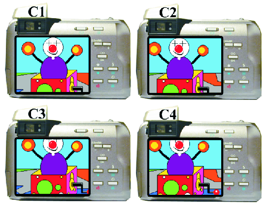
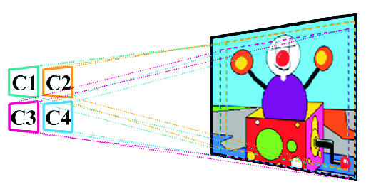
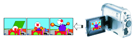
Figure 1: (a) Several cameras acquire still images of the same scene which
are combined to produce an HR image; (b) a video camera records a dynamic scene.
In motion based spatial RE the LR observed images are under-sampled and they are acquired by either multiple sensors imaging a single scene (Fig. 1(a)) or by a single sensor imaging a scene over a period of time (Fig. 1(b)). For static scenes the observations are related by global subpixel displacements (due, for example, to the relative positions of the cameras, and to camera motion, such as panning or zooming), while for dynamic scenes they are related by local sub-pixel displacements due to object motion, in addition to possibly global displacements. In both cases the objective again of SR is to utilize either the set of LR images (Fig. 1(a)) or a set of video frames (Fig. 1(b)) to generate an image of increased spatial resolution.
Increasing the resolution of the imaging sensor is clearly one way to increase the resolution of the acquired images. This solution, however, may not be feasible due to the increased associated cost and the fact that the shot noise increases during acquisition as the pixel size becomes smaller [135]. Furthermore, increasing the chip size to accommodate the larger number of pixels increases the capacitance, which in turn reduces the data transfer rate. Therefore, signal processing techniques, like the ones described in this book, provide a clear alternative for increasing the resolution of the acquired images.
There are various possible models in describing the systems depicted in Fig. 1. The block diagram of a general such model is shown in Fig. 2. According to it, there is a source discrete-space HR image which can represent the source continuous two-dimensional (2D) scene, that is, it resulted from the Nyquist sampling of the continuous 2D scene. This HR image is then warped and blurred before being downsampled. The warping represents the translation or rotation or any sophisticated mapping that is required to generate either the four still images shown in the example of Fig. 1(a), or a set of individual frames in the example of Fig. 1(b), from the original HR image. Registration is another term used to describe the estimation of the parameters of the warping model which will allow the re-alignment of the individual images or frames. The blur is modeling the response of the camera optics or the sensors or it can be due to the motion of the object or the out-of-focus acquisition of the scene. An interesting modeling question is the order in which these two operations —blurring and warping— are applied. Both resulting systems, the so called warp-blur and blur-warp models, have been used and are analyzed in detail in Chapter 3. Similarly, there are various ways to describe the downsampling block in Fig. 2, which will generate the aliased LR images of the original HR image. Finally, noise is added to the output of the system introducing the downsampling, resulting in the observed LR image. The noise component can model various elements in the imaging chain, such as, the misregistration error and the thermal or electronic noise, or the errors during storage or transmission.
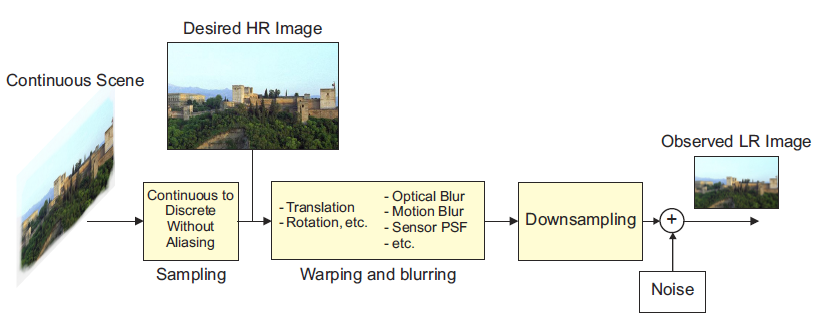 Figure 2: Block diagram of an SR system.
In the book we also consider the case when the available LR images have been compressed. In this case, one more block representing the compression system is added at the end of the block diagram of Fig. 2. Another noise component due to quantization needs to be considered in this case, which is typically considered to be the dominant noise component, especially for low bit-rates. As is clear from the block diagram of Fig. 2, in a typical SR problem there are a number of degradations that need to be ameliorated, in addition to increasing the resolution of the observations. The term RE might be therefore more appropriate in describing the type of problems we are addressing in this book.
Image restoration, a field very closely related to that of SR of images, started with the scientific work in the Space programs of the United States and the former Soviet Union [11, 116]. It could be said that the field of SR also started in the sky with the launching of Landsat satellites. These satellites imaged the same region on the Earth every 18 days. However, the observed scenes were not exactly the same since there were small displacements among them [190]. Since then, a wealth of research has considered modeling the acquisition of the LR images and provided solutions to the HR problem. Recent literature reviews are provided in [22, 26, 41, 85, 123]. More recent work, e.g., [108, 133, 134, 166] also addresses the HR problem when the available LR images are compressed using any of the numerous image and video compression standards or a proprietary technique. In the book we address both cases of uncompressed and compressed LR data.
To illustrate the effectiveness of SR methods consider, for example, Fig. 3. In Fig. 3(a) four LR images of the same scene are shown. These observed images are under-sampled and they are related by global sub-pixel shifts which are assumed to be known. In Fig. 3(b) the HR image obtained by the smart size filter in Corel® Paint Shop Pro® X on one of the observed images is shown. In Fig. 3(c) the super-resolved image obtained with the use of the algorithm in [193] (to be described later) that combines the four LR images is shown. As can be seen, a considerable improvement can be obtained by using the information contained in all four images.
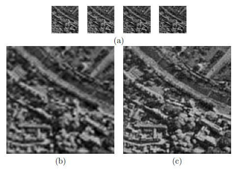
Figure 3: (a) Observed LR images with global sub-pixel displacement among them; (b) Upsampled image of the top left LR image using the Corel® Paint Shop Pro® X smart size filter; (c) HR image obtained by combining the information in the LR observations using the algorithm in [193].
Problem Description and Bayesian Formulation
Figure 1 provides a graphical description of the video spatial Super Resolution (SR) problem, see [1]. As shown in the figure, we denote by the vector fk the (lexicographically) ordered intensities of the k-th High Resolution (HR) frame. A set of frames can be similarly ordered to form a new vector f. We denote by the vector gk the ordered intensities of the k-th Low Resolution (LR) frame. Similarly, the set of LR frames corresponding to the HR frames in f can be ordered to form the vector g.
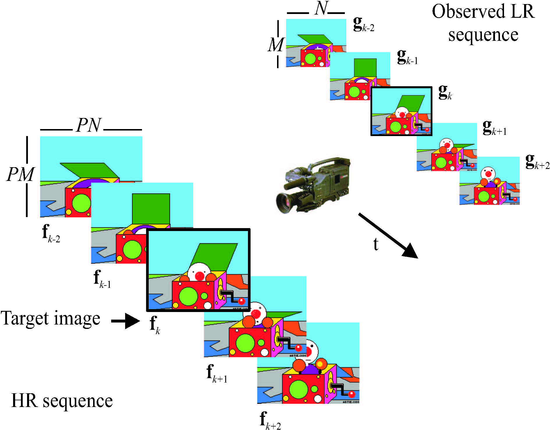
Figure 4: LR video acquisition model for the uncompressed case. The process to obtain the HR images from the LR ones has to account for sensor and optical distortions, motion, nonzero aperture time, downsampling, and noise. The HR images are denoted by f and the LR observations by g. The target HR image is denoted by fk.
We denote by the vector dl,k the warping model parameters in mapping frame fk to fl. The vector dl,k contains the motion parameters for compensating frame fl from frame fk (this means that each pixel value in frame fl can be predicted through the motion dl,k from a pixel in frame fk). The motion vectors have sub-pixel accuracy and therefore the pixel values in fk need to be interpolated in carrying out the motion compensation. A set of vectors dl,k can be ordered to form the vector d. This same model and notation can be applied to the SR problem of still images. In this case, there is only one HR image f and a number of HR observations gk, which are related by LR warp parameters or shifts d.
A fundamental principle of the Bayesian philosophy is to regard all parameters and observable variables as unknown stochastic quantities, assigning probability distributions based on subjective beliefs. Thus, in SR the original HR image fk, the motion vectors d, and the vector containing the blurring functions in the acquisition process h are all treated as samples of random fields, with corresponding prior distributions that model our knowledge about the nature of the original HR image, motion vectors, and blurring functions. The observation g, which is a function of fk, d,and h, is also treated as a sample of a random field, with corresponding conditional distribution that models the process to obtain g from fk, d, and h. These distributions depend on parameters which will be denoted by Ω.
The joint distribution modeling the relationship between the observed data and the unknown quantities of the SR problem becomes
P(Ω, f, d, h, g)= P(Ω)P(fk, d, h|Ω)P(g|fk, d, h, Ω),
Once the modeling has been completed, Bayesian inference, that is, the estimation of all the unknown in the SR problem, is performed finding and using the posterior distribution
P(Ω, f, d, h|g)= P(Ω, f, d, h, g) /
P(g).
Goals of the Project
According to the above de nition of the SR problem based on its Bayesian modelling and inference, the project was structured in the following tasks with their correspondent starting and ending dates:
- Task 1: Modelling of blur and warping. M1-M16.
- Tasks 2 and 3: Modelling of the underlying HR image, for general and specific domain priors. M1-M16.
- Tasks 4 and 5: Use of the models developed in Task 1-3 to carry out inference for general and specific domain priors. M17-M32.
- Task 6: Creation and maintenance of a database of images. M1-M32.
- Task 7: Comparison of approaches, dissemination of results, images, and Matlab® software. M33-M36.
The ultimate goals of all these tasks are: to develop methods to estimate all the unknown in a SR problem and to publicly provide a friendly Matlab® software application implementing the estimation task.